 This blog post is the fourth part of the series on Clustering with Dirichlet Process Mixture Models. In previous articles we discussed the Finite Dirichlet Mixture Models and we took the limit of their model for infinite k clusters which led us to the introduction of Dirichlet Processes. As we saw, our target is to build a mixture model which does not require us to specify the number of k clusters/components from the beginning. After presenting different representations of Dirichlet Processes, it is now time to actually use DPs to construct an infinite Mixture Model that enable us to perform clustering. The target of this article is to define the Dirichlet Process Mixture Models and discuss the use of Chinese Restaurant Process and Gibbs Sampling. If you have not read the previous posts, it is highly recommended to do so as the topic is a bit theoretical and requires good understanding on the construction of the model.
Update: The Datumbox Machine Learning Framework is now open-source and free to download. Check out the package com.datumbox.framework.machinelearning.clustering to see the implementation of Dirichlet Process Mixture Models in Java.
Using Dirichlet Processes allows us to have a mixture model with infinite components which can be thought as taking the limit of the finite model for k to infinity. Let’s assume that we have the following model:
![]()
![]()
![]()
Equation 1: Dirichlet Process Mixture Model
Where G is defined as ![]() and
and ![]() used as a short notation for
used as a short notation for ![]() which is a delta function that takes 1 if
which is a delta function that takes 1 if ![]() and 0 elsewhere. The θi are the cluster parameters which are sampled from G. The generative distribution F is configured by cluster parameters θi and is used to generate xi observations. Finally we can define a Density distribution
and 0 elsewhere. The θi are the cluster parameters which are sampled from G. The generative distribution F is configured by cluster parameters θi and is used to generate xi observations. Finally we can define a Density distribution ![]() which is our mixture distribution (countable infinite mixture) with mixing proportions
which is our mixture distribution (countable infinite mixture) with mixing proportions ![]() and mixing components
and mixing components ![]() .
.
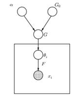
Figure 1: Graphical Model of Dirichlet Process Mixture Model
Above we can see the equivalent Graphical Model of the DPMM. The G0 is the base distribution of DP and it is usually selected to be conjugate prior to our generative distribution F in order to make the computations easier and make use of the appealing mathematical properties. The α is the scalar hyperparameter of Dirichlet Process and affects the number of clusters that we will get. The larger the value of α, the more the clusters; the smaller the α the fewer clusters. We should note that the value of α expresses the strength of believe in G0. A large value indicates that most of the samples will be distinct and have values concentrated on G0. The G is a random distribution over Θ parameter space sampled from the DP which assigns probabilities to the parameters. The θi is a parameter vector which is drawn from the G distribution and contains the parameters of the cluster, F distribution is parameterized by θi and xi is the data point generated by the Generative Distribution F.
It is important to note that the θi are elements of the Θ parameter space and they “configure” our clusters. They can also be seen as latent variables on xi which tell us from which component/cluster the xi comes from and what are the parameters of this component. Thus for every xi that we observe, we draw a θi from the G distribution. With every draw the distribution changes depending on the previous selections. As we saw in the Blackwell-MacQueen urn scheme the G distribution can be integrated out and our future selections of θi depend only on G0: ![]() . Estimating the parameters θi from the previous formula is not always feasible because many implementations (such as Chinese Restaurant Process) involve the enumerating through the exponentially increasing k components. Thus approximate computational methods are used such as Gibbs Sampling. Finally we should note that even though the k clusters are infinite, the number of active clusters is
. Estimating the parameters θi from the previous formula is not always feasible because many implementations (such as Chinese Restaurant Process) involve the enumerating through the exponentially increasing k components. Thus approximate computational methods are used such as Gibbs Sampling. Finally we should note that even though the k clusters are infinite, the number of active clusters is ![]() . Thus the θi will repeat and exhibit a clustering effect.
. Thus the θi will repeat and exhibit a clustering effect.
The model defined in the previous segment is mathematically solid, nevertheless it has a major drawback: for every new xi that we observe, we must sample a new θi taking into account the previous values of θ. The problem is that in many cases, sampling these parameters can be a difficult and computationally expensive task.
An alternative approach is to use the Chinese Restaurant Process to model the latent variables zi of cluster assignments. This way instead of using θi to denote both the cluster parameters and the cluster assignments, we use the latent variable zi to indicate the cluster id and then use this value to assign the cluster parameters. As a result, we no longer need to sample a θ every time we get a new observation, but instead we get the cluster assignment by sampling zi from CRP. With this scheme a new θ is sampled only when we need to create a new cluster. Below we present the model of this approach:
![]()
![]()
![]()
Equation 2: Mixture Model with CRP
The above is a generative model that describes how the data xi and the clusters are generated. To perform the cluster analysis we must use the observations xi and estimate the cluster assignments zi.
Unfortunately since Dirichlet Processes are non-parametric, we can’t use EM algorithm to estimate the latent variables which store the cluster assignments. In order to estimate the assignments we will use the Collapsed Gibbs Sampling.
The Collapsed Gibbs Sampling is a simple Markov Chain Monte Carlo (MCMC) algorithm. It is fast and enables us to integrate out some variables while sampling another variable. Nevertheless this algorithms requires us to select a G0 which is a conjugate prior of F generative distribution in order to be able to solve analytically the equations and be able to sample directly from ![]() .
.
The steps of the Collapsed Gibbs Sampling that we will use to estimate the cluster assignments are the following:
In the next article we will focus on how to perform cluster analysis by using Dirichlet Process Mixture models. We will define two different Dirichlet Process Mixture Models which use the Chinese Restaurant Process and the Collapsed Gibbs Sampling in order to perform clustering on continuous datasets and documents.
My name is Vasilis Vryniotis. I'm a Machine Learning Engineer and a Data Scientist. Learn more


")


Datumbox offers an open-source Machine Learning Framework and an easy to use and powerful API.
Subscribe to our newsletter and get our latest news!
2013-2026 © Datumbox. All Rights Reserved. Privacy Policy | Terms of Use


very useful
you mentioned we draw theta(i) from G distribution for the following equation, theta(i)|G~G. May I know why we need to write |G in the equation which becomes theta(i) from G distribution given G?