 This article is the third part of the series on Clustering with Dirichlet Process Mixture Models. The previous time we defined the Finite Mixture Model based on Dirichlet Distribution and we posed questions on how we can make this particular model infinite. We briefly discussed the idea of taking the limit of the model when the k number of clusters tends to infinity but as we stressed the existence of such an object is not trivial (in other words, how do we actually “take the limit of a model”?). As a reminder, the reason why we want to take make k infinite is because in this way we will have a non-parametric model which does not require us to predefine the total number of clusters within the data.
Update: The Datumbox Machine Learning Framework is now open-source and free to download. Check out the package com.datumbox.framework.machinelearning.clustering to see the implementation of Dirichlet Process Mixture Models in Java.
Even though our target is to build a model which is capable of performing clustering on datasets, before that we must discuss about Dirichlet Processes. We will provide both the strict mathematical definitions and the more intuitive explanations of DP and we will discuss ways to construct the process. Those constructions/representations can be seen as a way to find occurrences of Dirichlet Process in “real life”.
Despite the fact that I tried to adapt my research report in such a way so that these blog posts are easier to follow, it is still important to define the necessary mathematical tools and distributions before we jump into using the models. Dirichlet Process models are a topic of active research, but they do require having a good understanding of Statistics and Stochastic Processes before using them. Another problem is that as we will see in this article, Dirichlet Processes can be represented/constructed with numerous ways. As a result several academic papers use completely different notation/conventions and examine the problem from different points of view. In this post I try to explain them as simple as possible and use the same notation. Hopefully things will become clearer with the two upcoming articles which focus on the definition of Dirichlet Process Mixture Models and on how to actually use them to perform cluster analysis.
A Dirichlet process over a Θ space is a stochastic process. It is a probability distribution over “probability distributions over Θ space” and a draw from it is a discrete distribution. More formally a Dirichlet Distribution is a distribution over probability measures. A probability measure is a function of subsets of space Θ to [0,1]. G is a DP distributed random probability measure, denoted as ![]() , if for any partition (A1,…An) of space Θ we have that
, if for any partition (A1,…An) of space Θ we have that ![]() .
.
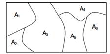
Figure 1: Marginals on finite partitions are Dirichlet distributed.
The DP has two parameters: The first one is the base distribution G0 which serves like a mean ![]() . The second one is the strength parameter α which is strictly positive and serves like inverse-variance
. The second one is the strength parameter α which is strictly positive and serves like inverse-variance ![]() . It determines the extent of the repetition of the values of the output distribution. The higher the value of a, the smaller the repetition; the smaller the value, the higher the repetition of the values of output distribution. Finally the Θ space is the parameter space on which we define the DP. Moreover the space Θ is also the definition space of G0 which is the same as the one of G.
. It determines the extent of the repetition of the values of the output distribution. The higher the value of a, the smaller the repetition; the smaller the value, the higher the repetition of the values of output distribution. Finally the Θ space is the parameter space on which we define the DP. Moreover the space Θ is also the definition space of G0 which is the same as the one of G.
A simpler and more intuitive way to explain a Dirichlet Process is the following. Suppose that we have a space Θ that can be partitioned in any finite way (A1,…,An) and a probability distribution G which assigns probabilities to them. The G is a specific probability distribution over Θ but there are many others. The Dirichlet Process on Θ models exactly this; it is a distribution over all possible probability distributions on space Θ. The Dirichlet process is parameterized with the G0 base function and the α concentration parameter. We can say that G is distributed according to DP with parameters α and G0 if the joint distribution of the probabilities that G assigns to the partitions of Θ follows the Dirichlet Distribution. Alternatively we can say that the probabilities that G assigns to any finite partition of Θ follows Dirichlet Distribution.
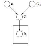
Figure 2: Graphical Model of Dirichlet Process
Finally above we can see the graphical model of a DP. We should note that α is a scalar hyperparameter, G0 is the base distribution of DP, G a random distribution over Θ parameter space sampled from the DP which assigns probabilities to the parameters and θi is a parameter vector which is drawn from the G distribution and it is an element of Θ space.
The Posterior Dirichlet Processes were discussed by Ferguson. We start by drawing a random probability measure G from a Dirichlet Process, ![]() . Since G is a probability distribution over Θ we can also sample from this distribution and draw independent identically distributed samples θ1,…, θn ~ G. Since draws from a Dirichlet Process are discrete distributions, we can represent
. Since G is a probability distribution over Θ we can also sample from this distribution and draw independent identically distributed samples θ1,…, θn ~ G. Since draws from a Dirichlet Process are discrete distributions, we can represent ![]() where
where ![]() is a short notation for
is a short notation for ![]() which is a delta function that takes 1 if
which is a delta function that takes 1 if ![]() and 0 elsewhere. An interesting effect of this is that since G is defined this way, there is a positive probability of different samples having the same value
and 0 elsewhere. An interesting effect of this is that since G is defined this way, there is a positive probability of different samples having the same value ![]() . As we will see later on, this creates a clustering effect that can be used to perform Cluster Analysis on datasets.
. As we will see later on, this creates a clustering effect that can be used to perform Cluster Analysis on datasets.
By using the above definitions and observations we want to estimate the posterior of the Dirichlet Process given the samples θ. Nevertheless since we know that ![]() and
and ![]() by using the Bayes Rules and the Conjugacy between Dirichlet and Multinomial we have that
by using the Bayes Rules and the Conjugacy between Dirichlet and Multinomial we have that ![]() and
and ![]() .
.
![]()
Equation 1: Posterior Dirichlet Process
This property is very important and it is used by the various DP representations.
In the previous segments we defined the Dirichlet Process and presented its theoretical model. One important question that we must answer is how do we know that such an object exists and how we can construct and represent a Dirichlet Process.
The first indications of existence was provided by Ferguson who used the Kolmogorov Consistency Theorem, gave the definition of a Dirichlet Process and described the Posterior Dirichlet Process. Continuing his research, Blackwell and MacQueen used the de Finetti’s Theorem to prove the existence of such a random probability measure and introduced the Blackwell-MacQueen urn scheme which satisfies the properties of Dirichlet Process. In 1994 Sethuraman provided an additional simple and direct way of constructing a DP by introducing the Stick-breaking construction. Finally another representation was provided by Aldous who introduced the Chinese Restaurant Process as an effective way to construct a Dirichlet Process.
The various Representations of the Dirichlet Process are mathematically equivalent but their formulation differs because they examine the problem from different points of view. Below we present the most common representations found in the literature and we focus on the Chinese Restaurant Process which provides a simple and computationally efficient way to construct inference algorithms for Dirichlet Process.
The Blackwell-MacQueen urn scheme can be used to represent a Dirichlet Process and it was introduced by Blackwell and MacQueen. It is based on the Pólya urn scheme which can be seen as the opposite model of sampling without replacement. In the Pólya urn scheme we assume that we have a non-transparent urn that contains colored balls and we draw balls randomly. When we draw a ball, we observe its color, we put it back in the urn and we add an additional ball of the same color. A similar scheme is used by Blackwell and MacQueen to construct a Dirichlet Process.
This scheme produces a sequence of θ1,θ2,… with conditional probabilities ![]() . In this scheme we assume that G0 is a distribution over colors and each θn represents the color of the ball that is placed in the urn. The algorithm is as follows:
. In this scheme we assume that G0 is a distribution over colors and each θn represents the color of the ball that is placed in the urn. The algorithm is as follows:
· We start with an empty urn.
· With probability proportional to α we draw ![]() and we add a ball of this color in the urn.
and we add a ball of this color in the urn.
· With probability proportional to n-1 we draw a random ball from the urn, we observe its color, we place it back to the urn and we add an additional ball of the same color in the urn.
Previously we started with a Dirichlet Process and derived the Blackwell-MacQueen scheme. Now let’s start reversely from the Blackwell-MacQueen scheme and derive the DP. Since θi were drawn in an iid manner from G, their joint distribution will be invariant to any finite permutations and thus they are exchangeable. Consequently by using the de Finetti’s theorem, we have that there must exist a distribution over measures to make them iid and this distribution is the Dirichlet Process. As a result we prove that the Blackwell-MacQueen urn scheme is a representation of DP and it gives us a concrete way to construct it. As we will see later, this scheme is mathematically equivalent to the Chinese Restaurant Process.
The Stick-breaking construction is an alternative way to represent a Dirichlet Process which was introduced by Sethuraman. It is a constructive way of forming the ![]() distribution and uses the following analogy: We assume that we have a stick of length 1, we break it at position β1 and we assign π1 equal to the length of the part of the stick that we broke. We repeat the same process to obtain π2, π3,… etc; due to the way that this scheme is defined we can continue doing it infinite times.
distribution and uses the following analogy: We assume that we have a stick of length 1, we break it at position β1 and we assign π1 equal to the length of the part of the stick that we broke. We repeat the same process to obtain π2, π3,… etc; due to the way that this scheme is defined we can continue doing it infinite times.
Based on the above the πk can be modeled as ![]() , where the
, where the ![]() while as in the previous schemes the θ are sampled directly by the Base distribution
while as in the previous schemes the θ are sampled directly by the Base distribution ![]() . Consequently the G distribution can be written as a sum of delta functions weighted with πk probabilities which is equal to
. Consequently the G distribution can be written as a sum of delta functions weighted with πk probabilities which is equal to ![]() . Thus the Stick-breaking construction gives us a simple and intuitively way to construct a Dirichlet Process.
. Thus the Stick-breaking construction gives us a simple and intuitively way to construct a Dirichlet Process.
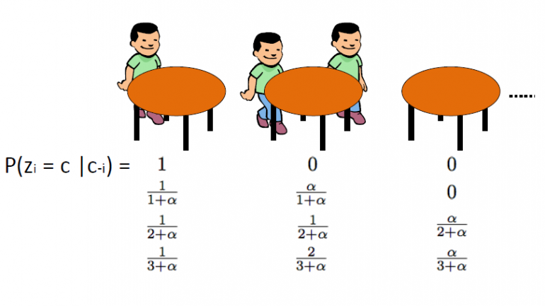
The Chinese Restaurant Process, which was introduced by Aldous, is another effective way to represent a Dirichlet Process and it can be directly linked to Blackwell-MacQueen urn scheme. This scheme uses the following analogy: We assume that there is a Chinese restaurant with infinite many tables. As the customers enter the restaurant they sit randomly to any of the occupied tables or they choose to sit to the first available empty table.
The CRP defines a distribution on the space of partitions of the positive integers. We start by drawing θ1,…θn from Blackwell-MacQueen urn scheme. As we discussed in the previous segments, we expect to see a clustering effect and thus the total number of unique θ values k will be significantly less than n. Thus this defines a partition of the set {1,2,…,n} in k clusters. Consequently drawing from the Blackwell-MacQueen urn scheme induces a random partition of the {1,2,…,n} set. The Chinese Restaurant Process is this induced distribution over partitions. The algorithm is as follows:
· We start with an empty restaurant.
· The 1st customer sits always on 1st table
· The n+1th customer has 2 options:
o Sit on the 1st unoccupied table with probability ![]()
o Sit on any of the kth occupied tables with probability ![]()
where ![]() is the number of people sitting on that table
is the number of people sitting on that table
Where α is the dispersion value of DP and n is the total number of customers in the restaurant at a given time. The latent variable zi stores the table number of the ith customer and takes values from 1 to kn where kn is the total number of occupied tables when n customers are in the restaurant. We should note that the kn will always be less or equal to n and on average it is about ![]() . Finally we should note that the probability of table arrangement
. Finally we should note that the probability of table arrangement ![]() is invariant to permutations. Thus the zi is exchangeable which implies that tables with same size of customers have the same probability.
is invariant to permutations. Thus the zi is exchangeable which implies that tables with same size of customers have the same probability.
The Chinese Restaurant Process is strongly connected to Pólya urn scheme and Dirichlet Process. The CRP is a way to specify a distribution over partitions (table assignments) of n points and can be used as a prior on the space of latent variable zi which determines the cluster assignments. The CRP is equivalent to Pólya’s urn scheme with only difference that it does not assign parameters to each table/cluster. To go from CRP to Pólya’s urn scheme we draw ![]() for all tables k=1,2… and then for every xi which is grouped to table zi assign a
for all tables k=1,2… and then for every xi which is grouped to table zi assign a ![]() . In other words assign to the new xi the parameter θ of the table. Finally since we can’t assign the θ to infinite tables from the beginning, we can just assign a new θ every time someone sits on a new table. Due to all the above, the CRP can help us build computationally efficient algorithms to perform Cluster Analysis on datasets.
. In other words assign to the new xi the parameter θ of the table. Finally since we can’t assign the θ to infinite tables from the beginning, we can just assign a new θ every time someone sits on a new table. Due to all the above, the CRP can help us build computationally efficient algorithms to perform Cluster Analysis on datasets.
In this post, we discussed the Dirichlet Process and several ways to construct it. We will use the above ideas in the next article. We will introduce the Dirichlet Process Mixture Model and we will use the Chinese Restaurant Representation in order to construct the Dirichlet Process and preform Cluster Analysis. If you missed few points don’t worry as things will start becoming clearer with the next two articles.
I hope you found this post interesting. If you did, take a moment to share it on Facebook and Twitter. 🙂
My name is Vasilis Vryniotis. I'm a Machine Learning Engineer and a Data Scientist. Learn more


")


Datumbox offers an open-source Machine Learning Framework and an easy to use and powerful API.
Subscribe to our newsletter and get our latest news!
2013-2026 © Datumbox. All Rights Reserved. Privacy Policy | Terms of Use


Leave a Reply