Finite Mixture Model based on Dirichlet Distribution

• May 12, 2014
• Vasilis Vryniotis
• . 4 Comments

• Machine Learning & Statistics

This blog post is the second part of an article series on Dirichlet Process mixture models. In the previous article we had an overview of several Cluster Analysis techniques and we discussed some of the problems/limitations that rise by using them. Moreover we briefly presented the Dirichlet Process Mixture Models, we talked about why they are useful and we presented some of their applications.

Update: The Datumbox Machine Learning Framework is now open-source and free to download. Check out the package com.datumbox.framework.machinelearning.clustering to see the implementation of Dirichlet Process Mixture Models in Java.

The Dirichlet Process Mixture Models can be a bit hard to swallow at the beginning primarily because they are infinite mixture models with many different representations. Fortunately a good way to approach the subject is by starting from the Finite Mixture Models with Dirichlet Distribution and then moving to the infinite ones.

Consequently in this article I will briefly present some important distributions that we will need, we will use them to construct the Dirichlet Prior with Multinomial Likelihood model and then we will move to the Finite Mixture Model based on the Dirichlet Distribution.

1. Beta Distribution

The Beta distribution is a family of continuous distributions which is defined in the interval of [0,1]. It is parameterized by two positive parameters a and b and its form heavily depends upon the selection of those two parameters.

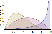
Figure 1: Beta Distribution for different a, b parameters

The Beta distribution is commonly used to model a distribution over probabilities and has the following probability density:

Equation 1: Beta PDF

Where Γ(x) is the gamma function and a, b the parameters of the distribution. Beta is commonly used as a distribution of probability values and gives us the likelihood that the modelled probability equals to a particular value P = p0. By its definition Beta distribution is able to model the probability of binary outcomes which take values true or false. The parameters a and b can be considered as the pseudocounts of success and failure respectively. Thus the Beta Distribution models the probability of success given a successes and b failures.

2. Dirichlet Distribution

The Dirichlet Distribution is the generalisation of Beta Distribution for multiple outcomes (or in other words it is used for events with multiple outcomes). It is parameterized with k parameters a_i which must be positive. Dirichlet Distribution equals to the Beta Distribution when the number of variables k = 2.

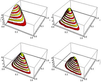
Figure 2: Dirichlet Distribution for various a_i parameters

The Dirichlet distribution is commonly used to model a distribution over probabilities and has the following probability density:

Equation 2: Dirichlet PDF

Where Γ(x) is the gamma function, the p_i take values in [0,1] and Σp_i=1. The Dirichlet distribution models the joint distribution of p_i and gives the likelihood of P₁=p₁,P₂=p₂,….,P_k-1=p_k-1 with P_k=1 – ΣP_i. As in the case of Beta, the a_i parameters can be considered as pseudocounts of the appearances of each i event. The Dirichlet distribution is used to model the probability of k rival events occurring and is often denoted as Dirichlet(a).

3. Dirichlet Prior with Multinomial Likelihood

As mentioned earlier the Dirichlet distribution can be seen as a distribution over probability distributions. In cases where we want to model the probability of k events occurring, a Bayesian approach would be to use Multinomial Likelihood and Dirichlet Priors .

Below we can see the graphical model of such a model.

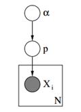
Figure 3: Graphical Model of Dirichlet Priors with Multinomial Likelihood

In the above graphical model, α is a k dimensional vector with the hyperparameters of Dirichlet priors, p is a k dimensional vector with the probability values and x_i is a scalar value from 1 to k which tells us which event has occurred. Finally we should note that the P follows the Dirichlet distribution parameterized with vector α and thus P ~ Dirichlet(α), while the x_i variables follow the Discrete distribution (Multinomial) parameterized with the p vector of probabilities. Similar hierarchical models can be used in document classification to represent the distributions of keyword frequencies for in different topics.

4. Finite Mixture Model with Dirichlet Distribution

By using Dirichlet Distribution we can construct a Finite Mixture Model which can be used to perform clustering. Let’s assume that we have the following model:

Equation 3: Finite Mixture Model with Dirichlet Distribution

The above model assumes the following: We have a dataset X with n observations and we want to perform cluster analysis on it. The k is a constant finite number which shows the number of clusters/components that we will use. The c_i variables store the cluster assignment of observation X_i, they take values from 1 to k and follow the Discrete Distribution with parameter p which are the mixture probabilities of the components. The F is the generative distribution of our X and it is parameterized with a parameter which depends on the cluster assignment of each observation. In total we have k unique parameters equal to the number of our clusters. The variable stores the parameters that parameterize the generative F Distribution and we assume that it follows a base G₀ distribution. The p variable stores the mixture percentages for every one of the k clusters and follows the Dirichlet with parameters α/k. Finally the α is a k dimensional vector with the hyperparameters (pseudocounts) of Dirichlet distribution [2].

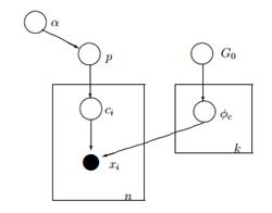
Figure 4: Graphical Model of Finite Mixture Model with Dirichlet Distribution

A simpler and less mathematical way to explain the model is the following. We assume that our data can be grouped in k clusters. Each cluster has its own parameters and those parameters are used to generate our data. The parameters are assumed to follow some distribution G₀. Each observation is represented with a vector x_i and a c_i value which indicates the cluster to which it belongs. Consequently the c_i can be seen as a variable which follows the Discrete Distribution with a parameter p which is nothing but the mixture probabilities, i.e. the probability of the occurrence of each cluster. Given that we handle our problem in a Bayesian way, we don’t treat the parameter p as a constant unknown vector. Instead we assume that the P follows Dirichlet which is parameterized by hyperparameters α/k.

5. Working with infinite k clusters

The previous mixture model allows us to perform unsupervised learning, follows a Bayesian approach and can be extended to have a hierarchical structure. Nevertheless it is a finite model because it uses a constant predefined k number of clusters. As a result it requires us to define the number of components before performing Cluster Analysis and as we discussed earlier in most applications this is unknown and can’t be easily estimated.

One way to resolve this is to imagine that k has a very large value which tends to infinity. In other words we can imagine the limit of this model when k tends to infinity. If this is the case, then we can see that despite that the number of clusters k is infinite, the actual number of clusters that are active (the ones that have at least one observation), can’t be larger than n (which is the total number of the observations in our dataset). In fact as we will see later, the number of active clusters will be significantly less than n and they will be proportional to .

Of course taking the limit of k to infinity is non-trivial. Several questions rise such as whether it is possible to take such a limit, how would this model look like and how can we construct and use such a model.

In the next article we will focus on exactly these questions: we will define the Dirichlet Process, we will present the various representations of DP and finally we will focus on the Chinese Restaurant Process which is an intuitive and efficient way to construct a Dirichlet Process.

I hope you found this post useful. If you did please take a moment to share the article on Facebook and Twitter. 🙂