 In the previous two machine learning tutorials, we examined the Naive Bayes and the Max Entropy classifiers. In this tutorial we will discuss the Multinomial Logistic Regression also known as Softmax Regression. Implementing Multinomial Logistic Regression in a conventional programming language such as C++, PHP or JAVA can be fairly straightforward despite the fact that an iterative algorithm would be required to estimate the parameters of the model.
Update: The Datumbox Machine Learning Framework is now open-source and free to download. Check out the package com.datumbox.framework.machinelearning.classification to see the implementation of SoftMax Regression Classifier in Java.
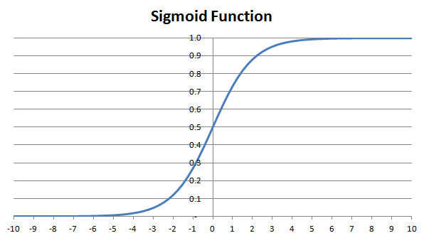
The Multinomial Logistic Regression, also known as SoftMax Regression due to the hypothesis function that it uses, is a supervised
learning algorithm which can be used in several problems including text classification. It is a regression model which generalizes the logistic regression to classification problems where the output can take more than two possible values. We should note that Multinomial Logistic Regression is closely related to MaxEnt algorithm because it uses the same activation functions. Nevertheless in this article we will present the method in a different context than we did on Max Entropy tutorial.
Multinomial Logistic Regression requires significantly more time to be trained comparing to Naive Bayes, because it uses an iterative algorithm to estimate the parameters of the model. After computing these parameters, SoftMax regression is competitive in terms of CPU and memory consumption. The Softmax Regression is preferred when we have features of different type (continuous, discrete, dummy variables etc), nevertheless given that it is a regression model, it is more vulnerable to multicollinearity problems and thus it should be avoided when our features are highly correlated.
Similarly to Max Entropy, we will present the algorithm in the context of document classification. Thus we will use the contextual information of the document in order to categorize it to a certain class. Let our training dataset consist of m (xi,yi) pairs and let k be the number of all possible classes. Also by using the bag-of-words framework let {w1,…,wn} be the set of n words that can appear within our texts.
The model of SoftMax regression requires the estimation of a coefficient theta for every word and category combination. The sign and the value of this coefficient show whether the existence of the particular word within a document has a positive or negative effect towards its classification to the category. In order to build our model we need to estimate the 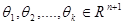 parameters. (Note that the θi vector stores the coefficients of ith category for each of the n words, plus 1 for coefficient of the intercept term).
In accordance with what we did previously for Max Entropy, all the documents within our training dataset will be represented as vectors with 0s and 1s that indicate whether each word of our vocabulary exists within the document. In addition, all vectors will include an additional “1” element for the intercept term.
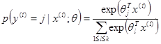
In Softmax Regression the probability given a document x to be classified as y is equal to:
 [1]
[1]
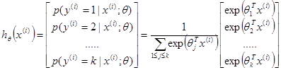
Thus given that we have estimated the aforementioned θ parameters and given a new document x, our hypothesis function will need to estimate the above probability for each of the k possible classes. Thus the hypothesis function will return a k dimensional vector with the estimated probabilities:
 [2]
[2]
By using the “maximum a posteriori” decision rule, when we classify a new document we will select the category with the highest probability.
In our Multinomial Logistic Regression model we will use the following cost function and we will try to find the theta parameters that minimize it:
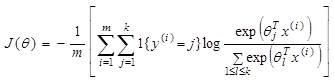 [3]
[3]
Unfortunately, there is no known closed-form way to estimate the parameters that minimize the cost function and thus we need to use an iterative algorithm such as gradient descent. The iterative algorithm requires us estimating the partial derivative of the cost function which is equal to:
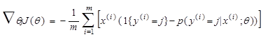 [4]
[4]
By using the batch gradient descent algorithm we estimate the theta parameters as follows:
1. Initialize vector θj with 0 in all elements

2. Repeat until convergence {

            θj <- θj - α  (for every j)

}
After estimating the θ parameters, we can use our model to classify new documents. Finally we should note that as we discussed in a previous article, using the Gradient Descent “as is” is never a good idea. Extending the algorithm to adapt learning rate and normalizing the values before performing the iterations are ways to improve convergence and speed up the execution.
Did you like the article? Please take a minute to share it on Twitter. 🙂
My name is Vasilis Vryniotis. I'm a Machine Learning Engineer and a Data Scientist. Learn more


")
Datumbox offers an open-source Machine Learning Framework and an easy to use and powerful API.
Subscribe to our newsletter and get our latest news!
2013-2026 © Datumbox. All Rights Reserved. Privacy Policy | Terms of Use


Thanks for the post!
Hi,
Thanks for explanation. But could you go more in detail about finding the gradient? I couldn’t understand the math of indicator function. When I find gradient, the prediction term is also multiplying with indicator function. Some more detail step would really solve my question.
Thanks in advance. Sorry for asking dumb question!