 In this tutorial we will discuss about Naive Bayes text classifier. Naive Bayes is one of the simplest classifiers that one can use because of the simple mathematics that are involved and due to the fact that it is easy to code with every standard programming language including PHP, C#, JAVA etc.
Update: The Datumbox Machine Learning Framework is now open-source and free to download. Check out the package com.datumbox.framework.machinelearning.classification to see the implementation of Naive Bayes Classifier in Java.
Note that some of the techniques described below are used on Datumbox’s Text Analysis service and they power up our API.
The Naive Bayes classifier is a simple probabilistic classifier which is based on Bayes theorem with strong and naïve independence assumptions. It is one of the most basic text classification techniques with various applications in email spam detection, personal email sorting, document categorization, sexually explicit content detection, language detection and sentiment detection. Despite the naïve design and oversimplified assumptions that this technique uses, Naive Bayes performs well in many complex real-world problems.
Even though it is often outperformed by other techniques such as boosted trees, random forests, Max Entropy, Support Vector Machines etc, Naive Bayes classifier is very efficient since it is less computationally intensive (in both CPU and memory) and it requires a small amount of training data. Moreover, the training time with Naive Bayes is significantly smaller as opposed to alternative methods.
Naive Bayes classifier is superior in terms of CPU and memory consumption as shown by Huang, J. (2003), and in several cases its performance is very close to more complicated and slower techniques.
You can use Naive Bayes when you have limited resources in terms of CPU and Memory. Moreover when the training time is a crucial factor, Naive Bayes comes handy since it can be trained very quickly. Indeed Naive Bayes is usually outperformed by other classifiers, but not always! Make sure you test it before you exclude it from your research. Keep in mind that the Naive Bayes classifier is used as a baseline in many researches.
There are several Naive Bayes Variations. Here we will discuss about 3 of them: the Multinomial Naive Bayes, the Binarized Multinomial Naive Bayes and the Bernoulli Naive Bayes. Note that each can deliver completely different results since they use completely different models.
Usually Multinomial Naive Bayes is used when the multiple occurrences of the words matter a lot in the classification problem. Such an example is when we try to perform Topic Classification. The Binarized Multinomial Naive Bayes is used when the frequencies of the words don’t play a key role in our classification. Such an example is Sentiment Analysis, where it does not really matter how many times someone mentions the word “bad” but rather only the fact that he does. Finally the Bernoulli Naive Bayes can be used when in our problem the absence of a particular word matters. For example Bernoulli is commonly used in Spam or Adult Content Detection with very good results.
As stated earlier, the Naive Bayes classifier assumes that the features used in the classification are independent. Despite the fact that this assumption is usually false, analysis of the Bayesian classification problem has shown that there are some theoretical reasons for the apparently unreasonable efficacy of Naive Bayes classifiers as Zhang (2004) shown. It can be proven (Manning et al, 2008) that even though the probability estimates of Naive Bayes are of low quality, its classification decisions are quite good. Thus, despite the fact that Naive Bayes usually over estimates the probability of the selected class, given that we use it only to make the decision and not to accurately predict the actual probabilities, the decision making is correct and thus the model is accurate.
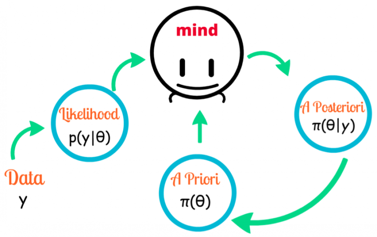
In a text classification problem, we will use the words (or terms/tokens) of the document in order to classify it on the appropriate class. By using the “maximum a posteriori (MAP)” decision rule, we come up with the following classifier:
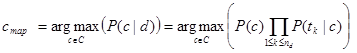
Where tk are the tokens (terms/words) of the document, C is the set of classes that is used in the classification,  the conditional probability of class c given document d,
  the prior probability of class c and
  the conditional probability of token tk given class c.
This means that in order to find in which class we should classify a new document, we must estimate the product of the probability of each word of the document given a particular class (likelihood), multiplied by the probability of the particular class (prior). After calculating the above for all the classes of set C, we select the one with the highest probability.
Due to the fact that computers can handle numbers with specific decimal point accuracy, calculating the product of the above probabilities will lead to float point underflow. This means that we will end up with a number so small, that will not be able to fit in memory and thus it will be rounded to zero, rendering our analysis useless. To avoid this instead of maximizing the product of the probabilities we will maximize the sum of their logarithms:

Thus instead of choosing the class with the highest probability we choose the one with the highest log score. Given that the logarithm function is monotonic, the decision of MAP remains the same.
The last problem that we should address is that if a particular feature/word does not appear in a particular class, then its conditional probability is equal to 0. If we use the first decision method (product of probabilities) the product becomes 0, while if we use the second (sum of their logarithms) the log(0) is undefined. To avoid this, we will use add-one or Laplace smoothing by adding 1 to each count:
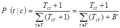
Where B’ is equal to the number of the terms contained in the vocabulary V.
Let’s examine three common Naive Bayes variations which differ on the way that they calculate the conditional probabilities of each feature and on the scoring of each category.
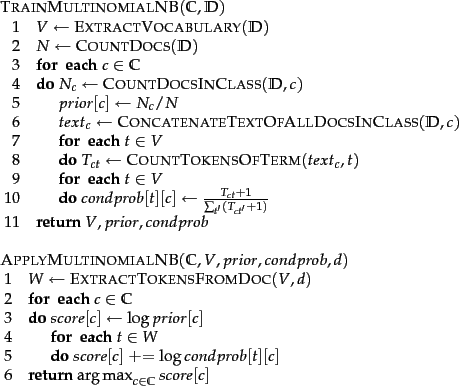
This variation, as described by Manning et al (2008), estimates the conditional probability of a particular word/term/token given a class as the relative frequency of term t in documents belonging to class c:
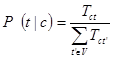
Thus this variation takes into account the number of occurrences of term t in training documents from class c, including multiple occurrences.
Both the training and the testing algorithms are presented below in the form of pseudo code:
This variation, as described by Dan Jurafsky, is identical to the Multinomial Naive Bayes model with only difference that instead of measuring all the occurrences of the term t in the document, it measures it only once. The reasoning behind this is that the occurrence of the word matters more than the word frequency and thus weighting it multiple times does not improve the accuracy of the model.
Both the training and the testing algorithms remain the same with only exception that instead of using multiple occurrences we clip all word counts in each document at 1.
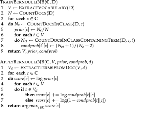
The Bernoulli variation, as described by Manning et al (2008), generates a Boolean indicator about each term of the vocabulary equal to 1 if the term belongs to the examining document and 0 if it does not. The model of this variation is significantly different from Multinomial not only because it does not take into consideration the number of occurrences of each word, but also because it takes into account the non-occurring terms within the document. While in Multinomial model the non-occurring terms are completely ignored, in Bernoulli model they are factored when computing the conditional probabilities and thus the absence of terms is taken into account.
Both the training and the testing algorithms are presented below:
Bernoulli model is known to make many mistakes while classifying long documents, primarily because it does not take into account the multiple occurrences of the words. Moreover we should note that it is particularly sensitive to the presence of noisy features.
If you are confused by all the statistics and maths, don’t worry! Datumbox made it simple to use Machine Learning from your software. Just sign-up for a free account and start using our easy-to-use REST Machine Learning API in no time.
Did you like the article? Please take a minute to share it on Twitter. 🙂
My name is Vasilis Vryniotis. I'm a Machine Learning Engineer and a Data Scientist. Learn more


Datumbox offers an open-source Machine Learning Framework and an easy to use and powerful API.
Subscribe to our newsletter and get our latest news!
2013-2026 © Datumbox. All Rights Reserved. Privacy Policy | Terms of Use


Hi Vasilis,
I was reading your blog today for the first time. Your insights to machine learning problems are very impressive and you are able to explain concepts very clearly.
Thank you for doing this!
Hi vasilis,
you have given a good explanation but you used the Multinomial navies for the sentiment analysis in classifier code example of Datumboxframe work but in this blog post you said Binarized Multinomial Naive Bayes is used for sentiment analysis can I know why you used Multinomial navies instead of Binarized Multinomial?
hello,
there’s sentiment package in R, where it is using algorithm = naive bayes. so i want to understand how it works over there.
Hi
Your article gives all details in one go
What if the test document contains words not in the vocabulary which was created during training phase?
Thank you for this excellent overview of Naive Bayes classification, Vasilis!